A/B Testing Statistical Significance: Sample Size Calculator Guide
Running an A/B test without understanding statistical significance is like flipping a coin and calling it strategy. You might get lucky, but you’re not making data-driven decisions. This guide breaks down the math behind valid A/B tests—and gives you the formulas to calculate sample size before you start.
What You’ll Learn
- What statistical significance actually means (and why 95% is the standard)
- How to calculate the sample size needed for your test
- The relationship between statistical power, effect size, and test duration
- How to interpret p-values without falling into common traps
- When to stop a test—and when stopping early destroys your data
The Core Concepts Behind A/B Testing Statistics
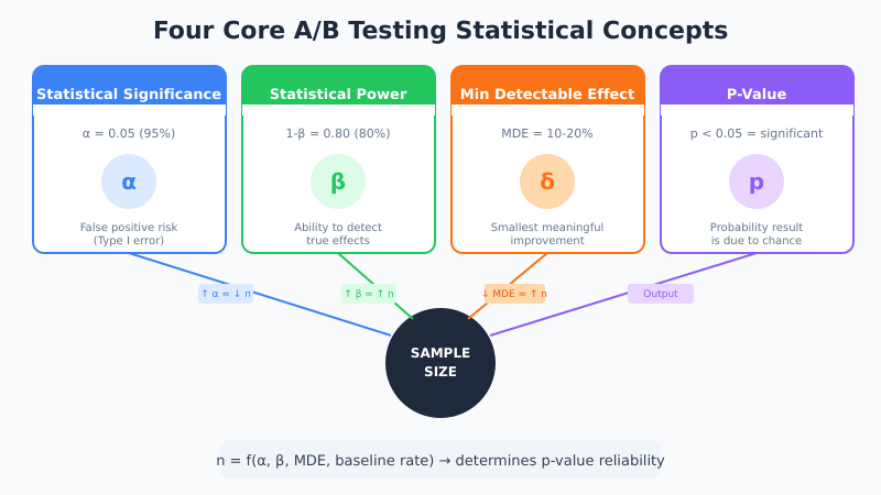
Before diving into calculators and formulas, you need to understand four interconnected concepts. These aren’t just academic terms—they directly determine whether your test results mean anything.
Statistical Significance (α)
Statistical significance measures the probability that your observed difference happened by pure chance. In other words, it answers: “If there’s actually no difference between A and B, how likely is it that I’d see results this extreme?”
The industry standard is 95% significance, which means a 5% chance (α = 0.05) of a false positive. However, this threshold isn’t magic. It’s a convention. For high-stakes decisions, you might want 99%. For quick iterations, 90% might suffice.
A statistically significant result doesn’t mean the result is important. It means the result is unlikely to be random noise.
Statistical Power (1-β)
Statistical power is the probability of detecting a real effect when one exists. Standard practice sets power at 80%, meaning you have an 80% chance of catching a true winner and a 20% chance of missing it (false negative).
Power and sample size are directly linked. Want higher power? You need more samples. Consequently, underpowered tests are one of the most common mistakes in CRO—you run a test, see no significant difference, and conclude there’s no effect. In reality, you simply didn’t have enough data to detect it.
Minimum Detectable Effect (MDE)
The minimum detectable effect is the smallest improvement you want your test to reliably detect. For example, if your baseline conversion rate is 3% and you set MDE at 10% relative lift, you’re looking to detect a change from 3% to 3.3%.
Smaller MDEs require larger sample sizes. Therefore, before running any test, ask yourself: “What’s the smallest lift that would justify implementing this change?” If a 2% lift isn’t worth the development effort, don’t design your test to detect it.
P-Value
The p-value represents the probability of observing your results (or more extreme results) if the null hypothesis is true. In simpler terms, it’s the chance that random variation produced your observed difference.
If p < 0.05, you reject the null hypothesis and declare significance. However, p-values are frequently misunderstood. A p-value of 0.03 doesn’t mean there’s a 97% chance your variant is better. It means there’s a 3% chance of seeing this result if both variants perform identically.
The Sample Size Formula Explained
The standard formula for calculating A/B test sample size per variation is:
n = (2 × σ² × (Z_α/2 + Z_β)²) / δ²Where:
| Symbol | Meaning | Typical Value |
|---|---|---|
| n | Sample size per variation | Calculated |
| σ² | Variance (p × (1-p) for conversions) | Based on baseline |
| Z_α/2 | Z-score for significance level | 1.96 for 95% |
| Z_β | Z-score for power | 0.84 for 80% |
| δ | Absolute effect size (MDE) | Your target lift |
For conversion rate tests, a simplified formula works well:
n = 16 × σ² / δ²This assumes 95% significance and 80% power. The number 16 comes from (1.96 + 0.84)² ≈ 7.84, doubled for two-tailed test.
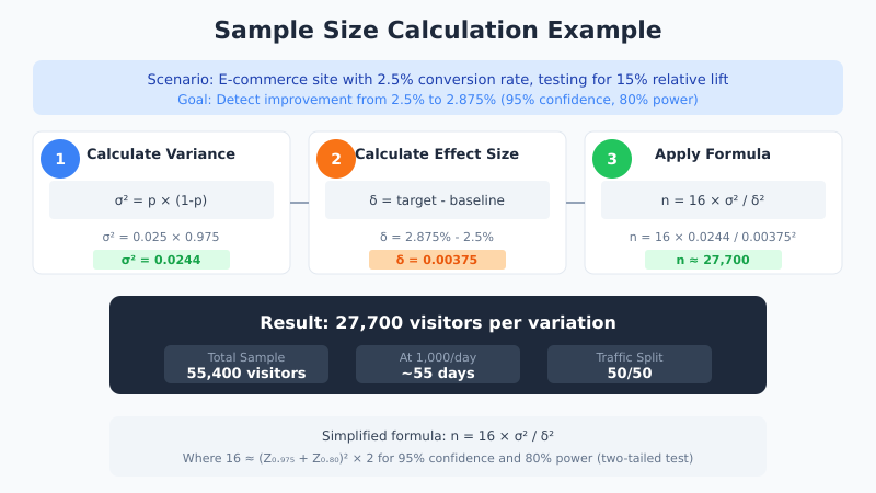
Practical Calculation Example
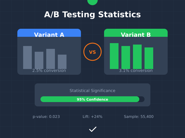
Let’s walk through a real scenario. Your e-commerce site has a 2.5% conversion rate, and you want to detect a 15% relative lift (from 2.5% to 2.875%).
Step 1: Calculate baseline variance
σ² = p × (1-p) = 0.025 × 0.975 = 0.0244Step 2: Calculate absolute effect size
δ = 2.875% - 2.5% = 0.375% = 0.00375Step 3: Apply the formula
n = 16 × 0.0244 / (0.00375)² = 16 × 0.0244 / 0.0000141 ≈ 27,700You need approximately 27,700 visitors per variation—or 55,400 total. At 1,000 daily visitors with 50/50 split, that’s roughly 55 days of testing.
How Sample Size Factors Interact
Understanding the relationships between variables helps you make smarter trade-offs. Here’s how each factor affects required sample size:
| If You… | Sample Size… | Trade-off |
|---|---|---|
| Increase confidence (95% → 99%) | Increases ~35% | Fewer false positives, longer tests |
| Increase power (80% → 90%) | Increases ~30% | Fewer false negatives, longer tests |
| Decrease MDE (20% → 10%) | Increases ~4× | Detect smaller effects, much longer tests |
| Higher baseline rate (2% → 5%) | Decreases | More conversions = more signal |
The MDE has the largest impact. Halving your minimum detectable effect quadruples your required sample size. Consequently, being realistic about what effect size matters is crucial for practical testing timelines.
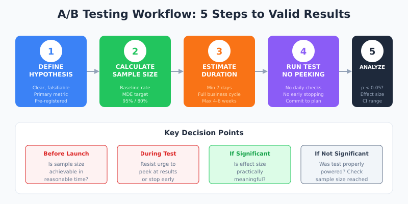
Step-by-Step: Running a Statistically Valid Test
Theory is useful, but execution matters more. Follow these steps to ensure your A/B tests produce trustworthy results.
Step 1: Define Your Hypothesis and Success Metric
Start with a clear, falsifiable hypothesis. Instead of “the new button might work better,” write: “Changing the CTA from ‘Submit’ to ‘Get My Quote’ will increase form completion rate by at least 15%.”
Additionally, define your primary metric upfront. Testing multiple metrics without pre-registration leads to cherry-picking significant results—a form of p-hacking that invalidates your conclusions. For structured hypothesis development, see our CRO Hypothesis Matrix guide.
Step 2: Calculate Required Sample Size
Before launching, determine how many visitors you need. Use these inputs:
- Baseline conversion rate: Pull from your analytics (minimum 2-4 weeks of data)
- Minimum detectable effect: The smallest lift worth implementing
- Significance level: 95% unless you have specific reasons to adjust
- Statistical power: 80% minimum, 90% for important tests
Use a sample size calculator or the formulas above. Document your calculation—you’ll need it to defend your results.
Step 3: Estimate Test Duration
Divide required sample size by your daily traffic to estimate duration. However, there are constraints:
- Minimum 7 days: Captures weekly behavior patterns (weekday vs. weekend)
- Minimum 2 business cycles: For B2B, this might mean 2-4 weeks
- Maximum 4-6 weeks: Longer tests risk external validity threats (seasonality, market changes)
If your calculation requires 90+ days, reconsider your MDE or test a higher-traffic page.
Step 4: Implement and Run Without Peeking
This step seems simple but causes the most problems. Once your test is live:
- Don’t check results daily: Early peeking inflates false positive rates
- Don’t stop at first significance: Random walks cross thresholds temporarily
- Don’t extend tests that “almost” reached significance: This is outcome-dependent stopping
Set your end date based on the sample size calculation. Run until you hit that date or sample size—whichever comes second.
Step 5: Analyze Results Correctly
When your test concludes, evaluate these criteria:
- Did you reach target sample size? If not, your test is underpowered.
- Is p < 0.05? If yes, the result is statistically significant.
- Is the effect size practically meaningful? Statistical significance ≠ business significance.
- Are confidence intervals useful? A 95% CI of [0.5%, 8%] is more informative than just “significant.”
Common Mistakes That Invalidate Your Tests
Even experienced testers make these errors. Understanding them helps you avoid wasted effort and misleading conclusions.
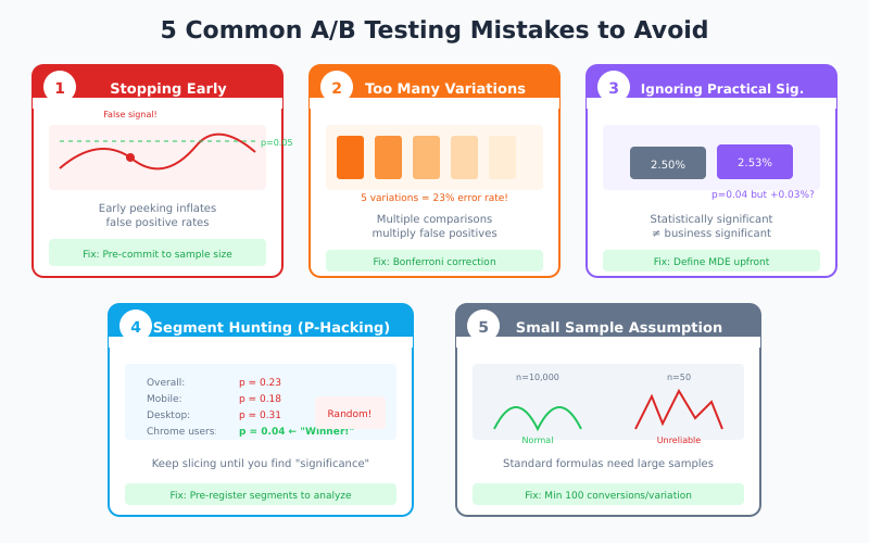
Mistake 1: Stopping Tests Early
You launch a test, check after 3 days, see p = 0.02, and declare a winner. The problem? With repeated checking, you’ll eventually hit significance by chance. This is called “optional stopping” and it dramatically inflates false positive rates.
Solution: Pre-commit to a fixed sample size or use sequential testing methods designed for continuous monitoring (like sequential analysis).
Mistake 2: Testing Too Many Variations
Testing 5 variations against a control seems efficient, but it increases false positive risk. With 5 comparisons at α = 0.05, your family-wise error rate jumps to ~23%.
Solution: Apply Bonferroni correction (α / number of comparisons) or run separate tests. For 5 variations, use α = 0.01 per comparison to maintain 5% overall error rate.
Mistake 3: Ignoring Practical Significance
A test shows 0.3% conversion lift with p = 0.04. Statistically significant, right? However, if implementing the change costs $50,000 in development, that 0.3% lift might never generate positive ROI.
Solution: Define your MDE based on business impact before testing. If it’s not worth detecting, don’t run the test.
Mistake 4: Segment Hunting
Your overall test shows no significance, so you slice the data by device, location, and user type until you find a “significant” segment. This is p-hacking—given enough segments, random variation will produce false positives.
Solution: Pre-register segments you plan to analyze. Post-hoc segment analysis is exploratory, not confirmatory—it generates hypotheses for future tests, not conclusions.
Mistake 5: Assuming Normality for Small Samples
Standard formulas assume normal distribution, which works for large samples via the Central Limit Theorem. For small samples (under 100 conversions), this assumption breaks down.
Solution: Use exact tests (Fisher’s exact test) for small samples, or ensure you have at least 100 conversions per variation before relying on z-tests.
Quick Reference: Sample Size Benchmarks
Use this table for rough estimates based on common scenarios. These assume 95% confidence and 80% power.
| Baseline Rate | 10% MDE | 15% MDE | 20% MDE | 25% MDE |
|---|---|---|---|---|
| 1% | 156,800 | 69,700 | 39,200 | 25,100 |
| 2% | 77,700 | 34,500 | 19,400 | 12,400 |
| 3% | 51,500 | 22,900 | 12,900 | 8,200 |
| 5% | 30,200 | 13,400 | 7,500 | 4,800 |
| 10% | 14,300 | 6,400 | 3,600 | 2,300 |
Values shown are per variation. Double for total test traffic (control + variant).
Tools and Calculators
While understanding the math matters, calculators save time. Here are the most reliable options:
| Tool | Best For | Features |
|---|---|---|
| Evan Miller’s Calculator | Quick calculations | Simple interface, instant results |
| Optimizely Calculator | Test planning | MDE visualization, clear explanations |
| AB Tasty Calculator | Duration estimates | Includes test duration based on traffic |
| CXL Calculator | Full analysis | Planning + significance testing |
| VWO Calculator | Bayesian analysis | Frequentist and Bayesian options |
Connecting Tests to Business Outcomes
Statistical rigor means nothing if tests don’t drive decisions. To maximize impact:
- Prioritize high-traffic pages: More traffic means faster tests and more statistical power
- Test closer to conversion: Checkout page changes impact revenue more directly than homepage tweaks
- Calculate expected value: A 10% chance of 50% lift might be worth more than a 90% chance of 2% lift
- Track downstream metrics: A conversion rate increase that tanks average order value isn’t a win
Connect your testing program to revenue impact. Track the cumulative value of implemented winning tests over time. For setting up proper conversion tracking, see our GA4 event and conversion tracking guide.
Bayesian vs. Frequentist: Which Approach?
Most calculators use frequentist statistics (the approach described above). However, Bayesian methods are gaining popularity. Here’s a quick comparison:
| Aspect | Frequentist | Bayesian |
|---|---|---|
| Output | P-value, confidence interval | Probability of being better |
| Sample size | Fixed, pre-calculated | Can be adaptive |
| Early stopping | Problematic without correction | Built-in handling |
| Interpretation | Often misunderstood | More intuitive |
| Prior knowledge | Not incorporated | Can use prior data |
Bayesian approaches tell you directly: “There’s a 94% probability that B is better than A.” This is often what people think p-values mean. For most business contexts, either approach works—consistency and proper execution matter more than the statistical framework.
Bottom Line
A/B testing statistical significance isn’t about complex math—it’s about intellectual honesty. Calculate your sample size before testing, commit to your methodology, and resist the temptation to peek or stop early. The formulas exist to protect you from seeing patterns in noise.
Remember these key points:
- 95% confidence and 80% power are standard thresholds, not magic numbers
- Minimum detectable effect has the largest impact on required sample size
- Pre-registration of hypotheses, metrics, and sample size prevents p-hacking
- Statistical significance doesn’t equal practical significance—always consider business impact
- When in doubt, run longer. Underpowered tests waste more time than slightly longer tests.
The goal isn’t to prove your hypothesis right. It’s to learn what actually works—even when the answer isn’t what you hoped for.